Quickstart Guide: Hyperparameter selection (and why theorists should care)

Training a neural network is a strange and mysterious process: a bewildering cavalcade of tensors is randomly initialized and subject to repeated gradient updates, and as a consequence of these simple operations, the whole thing learns. Meanwhile, before the process begins, you have to set your learning rate and some other fiddly knobs and dials. In comparison with the weights themselves, these hyperparameters might seem drab, technical and mundane; does a serious deep learning theorist really need to bother with them? It turns out the answer is emphatically “yes”: not only is the study of hyperparameters the easiest place for theory to make a practical impact, it’s also essential for the rest of the field, since any hyperparameter you can’t control for will interfere with your attempts to study anything else.

While most hyperparameters are still waiting for good theory, we understand a few. We’ll explain how theorists currently think about hyperparameters, list off the successes, and point out some frontiers. This chapter will be comparatively long, so we’ll start with a table of contents.

Classes of hyperparameter: optimization, architecture, and data

By hyperparameters, we mean all the numbers and choices that define our training process. Unlike the network parameters — the tensor weights optimized during training — hyperparameters are chosen at the start of training and don’t change. Together, the hyperparameters specify the optimization process, the architecture, and the preprocessing of the dataset. The choice of hyperparameters can make a big difference in model performance, and unless you have a smart way to choose them, it’s not uncommon to spend 10-100x the effort and compute you’d expend training the final model just optimizing hyperparameters. A little math can make this search much more methodical, and thus the science of hyperparameters is up and away the most practically impactful area of deep learning theory in 2025.

Even a simple neural network training procedure involves a dizzying array of hyperparameters. We will narrow in on only a few key hyperparameters for analytical study, but here at the outset, it’s worth enumerating a full list to get a sense of scope.

Hyperparameters can be grouped into three categories. First, optimization hyperparameters dictate how network parameters are initialized and respond to gradient.

1. The optimizer — SGD, Adam, Muon, or similar — fixes the functional form by which parameter gradients are turned into parameter updates.
2. The optimizer will have one or more hyperparameters — learning rate \(\eta\), momentum \(\mu\), weight decay \(\text{wd}\), tolerance \(\epsilon\), etc. — that enter as constants in the function above. These parameters affect the dynamics of optimization.
3. The batch size \(B\) and total step count \(T\) specify the amount of data in each gradient batch and the total number of batches to process.
4. The initialization scale \(\sigma\) for each layer specifies the size of parameters at init.

Optimization hyperparameters tend to be the most quantitative: many are real-valued numbers instead of choices from a discrete set. As a result, they are the most amenable to theoretical analysis and will receive most of our attention in this chapter.¹

Architectural hyperparameters dictate the structure of the network’s forward computation. These include the architecture type (MLP, CNN, transformer, etc.), the number of layers and their widths, the presence and location of norm layers, the choice of nonlinear activation function, the floating point resolution, and any other quirks of the network structure. The space of possible architectures is large and ill-defined, and it remains difficult to search over methodically. Of these hyperparameters, we will mostly discuss only network width, depth, and activation function, as these are the ones we currently know how to study.

Lastly, data hyperparameters include the choice of dataset, any cleaning, curation or tokenization procedures, any choice of curriculum, and any fine-tuning procedure. Though interesting and crucial, these choices are beyond the reach of current theory, and we will mostly omit them from the rest of the chapter.

How to deal with hyperparameters as a theorist

A practitioner concerned only with model performance can optimize hyperparameters numerically and forget about them. A theorist ought to be concerned with more than model performance, though, and should try to predict quantities that will be affected by these hyperparameters. For example, the loss (or sharpness, or feature change, etc.) after \(T\) steps will usually depend on the learning rate \(\eta\) (and a whole lot else), so any quantative prediction of the type we would like to make will depend explicitly on \(\eta\) and other hyperparameters. At first, this might seem to spell doom for our hopes for simple theory. What can we do?

There are two main answers. The first and easiest is to simply remove any hyperparameter you can. If you can do your study without a hyperparameter — momentum, say, or norm layers — do it; you can always add them back later, and your science will be clearer with fewer bells and whistles in the way. If your optimization process has a single unique minimizer reached no matter the learning rate, make sure you train for long enough to reach it. Doing this, you can usually reduce the problem to a few optimization hyperparameters (e.g. learning rate(s), batch size, and step count) and a few architectural hyperparameters (e.g. width, depth, activation function, init scale).

Recurring motif: hyperparameter scaling relationships

After removing all the hyperparameters you can, you should look for scaling relationships between your hyperparameters that let you reduce the effective number. For example, if you map \((\eta, T) \mapsto (\frac{1}{2} \eta, 2 T)\) — that is, you halve the learning rate and double the step count — then you approximately get the same training dynamics, so long as \(\eta\) was small enough to begin with. This “gradient flow” limit is very useful: unless finite stepsize effects are important for your study, you should work in it. In this limit, we only need to care about the “effective training time” \(\tau := \eta \cdot T\) and can forget \(\eta\) and \(T\) as independent quantities, so we’ve effectively reduced our number of hyperparameters by one.

The same is true of large width. In the previous chapter, we discussed how for a middle layer of a moderately wide MLP, the parameters should be initialized with scale \(\sigma \sim \frac{1}{\sqrt{\text{width}}}\). If you quadruple width, you should halve the init scale. If you also adjust the learning rate in accordance with \(\mu\)P, you can work in the large-width limit, and width vanishes as a hyperparameter. Unless finite width is important for your study, you should probably work mathematically in the large-width limit (and of course compare empirically to finite-width nets).

Since the experiments you run to match your theory won’t take place in an infinite or infinitesimal limit, we still have the question of how small is small enough (and ditto for “large”). Fortunately, numerical evidence suffices for this: divide \(\eta\) by another factor of 10, or multiply width by another factor of 10, and if the change in dynamics is negligible, you’re close enough to the limit.²

Almost all of our useful understanding of hyperparameters takes the form of hyperparameter scaling relationships.³ There are probably several important scaling relationships that remain to be worked out. After using all known relationships, you are usually still left with a handful of hyperparameters. The number of remaining hyperparameters often determines the difficulty of the calculation you have to do, so it’s a good idea to get it as low as possible.⁴

Without further ado, here are the hyperparameters we have theory for.

Width, initialization scale, and learning rate

This was mostly covered in the previous section. There’s essentially only one way to scale the layerwise init sizes and learning rates with model width such that you retain feature learning at large width. This scaling scheme is called the maximal-update parameterization, or \(\mu\)P.

• The original paper here is [Yang and Hu (2021)]. Most people find that [Yang et al. (2023)] gives a simpler exposition. The core idea here is essential; this is the only hyperparameter scaling relationship in this section that’s mandatory for doing or reading most modern deep learning theory.
• [Yang et al. (2022)]’s followup “\(\mu\)Transfer” paper showed that getting the scaling relationships here right can let you optimize your hyperparameters on a small model and scale them up to a large model, much like how civil engineers build scaled-down models to test the mechanics of proposed designs. This paper basically launched the modern study of hyperparameter scaling and is one of very few practically influential theory papers to date.

It’s worth noting that there are order-one constant prefactors at each layer that \(\mu\)P leaves undetermined. For example, \(\mu\)P tells us that the init scale for an intermediate layer should be such that \(\sigma_\text{eff} := \sigma * \sqrt{\text{width}}\) is an order-one, width-independent quantity, but it doesn’t tell us what the actual value should be. There is currently no theory that tells us what these should be.

The distinction between the “lazy” NTK regime and “rich” \(\mu\)P regime can be boiled down to a single hyperparameter \(\gamma\) that appears as an output multiplier on the network. This “richness” hyperparameter dictates how much hidden representations much change to effect an order-one change in the network output. This is an interesting hyperparameter to tune in its own right: \(\mu\)P prescribes that \(\gamma\) should be a width-independent constant, but the actual value of this constant significantly affects the dynamics of training. Smaller \(\gamma\) causes lazier training, weaker feature evolution, and more kernel-like training dynamics. At larger \(\gamma\), we start to see steps and plateaus in the loss curve. There’s a great deal of interesting and poorly-understood behavior in this “ultra-rich regime,” and some new ideas will be needed to understand it.

• [Atanasov et al. (2024)] found how the global learning rate should scale with \(\gamma\). The scaling exponents are different at large \(\gamma\).
  • This is a good first paper to read on the large-\(\gamma\) regime. If you can understand Figure 1, you have the important ideas.

The ultra-rich regime is essentially the same as the small-initialization or “saddle-to-saddle” regime, which has been studied since before \(\mu\)P.

• [Jacot et al. (2021)] coin the term “saddle-to-saddle” and describe the evolution of deep linear networks in this regime. They find a “greedy low-rank dynamics” and stepwise loss curves similar to those later seen in the ultra-rich regime. We will revisit saddle-to-saddle dynamics in the next chapter.

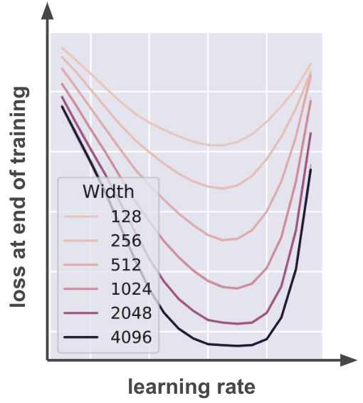
“Wider is better”

Whenever we take a limit and thereby simplify our model, we ought to ask whether we’ve lost any essential behavior. In the case of infinite width, it’s generally believed that infinite width nets outperform finite width nets on realistic tasks when the hyperparameters are properly tuned, which suggests that the core phenomena of deep learning we wish to explain are still there in the limit.

• [Yang et al. (2022)] found empirically that larger models perform strictly better when scaled up with \(\mu\)P.
• [Simon et al. (2024)] showed analytically that wider is better for a random feature model (i.e., a shallow net with the second layer trained).

Figure 1: This figure from Yang et al. (2022) shows both width transfer of optimal learning rate (loss minima fall on a vertical line) and “wider is better” (larger widths reach lower loss).

It’s very much an open question whether anything like this can be shown generally true in any setting where all layers are trained.

Answering this question would be quite impactful: it seems almost within reach, and it would open up a new type of question for analytical theory.

It’d also be interesting to know if there are counterexamples, even if they’re pretty handcrafted or unrealistic. Looking for counterexamples is probably an easier place to start than trying to prove the general theorem and might tell us if we’re barking up the wrong tree.

Depth

Network depth is also amenable to a treatment similar to that used to derive \(\mu\)P. Even before \(\mu\)P, though, we knew that large depth was a more finicky limit than large width.

• [Schoenholz et al. (2016)] found that infinite depth MLPs are ill-conditioned, even at infinite width. There are two different ways they can be ill-conditioned (”ordered” and “chaotic”), but both are bad for training.
  • It’s worth reading enough of this one that you can understand Figure 1 and could reproduce it if you had to. It’s important to get some intuitive feel for why infinite depth leads to ill-conditioned representations and gradients.
• [Hanin and Nica (2020)] found that finite-width corrections to the NTK of a randomly-initialized ReLU net scale like \(\exp(\text{depth/width})\). That is, you need \(\text{depth} \ll \text{width}\) to be in a deterministic “large width” regime. Otherwise, fluctuations due to the random init really matter.
  • You don’t need to follow the detailed calculation here, but it’s worth getting some intuition for why it’s true. Even a simple random matrix calculation works well enough to show this: take a product of \(L\) square random matrices of large dimension \([n \times n]\), and you’ll find that the singular spectrum of the product is close to deterministic when \(n \gg L\) and fluctuates otherwise.⁵

The moral of the above story is that you generally want to take width to infinity before you take depth to infinity, and you probably shouldn’t take depth to infinity if your model is a naive feedforward MLP.

The proper way to take depth to infinity involves a ResNet formulation with downweighted layers. Take a deep ResNet with \(L \gg 1\) layers. The activations will explode at init as you forward propagate through many layers unless you multiply each layer by a small factor so the total accumulated change remains order one (or, more properly, the same order as you’d get from one regular ResNet layer).

• [Bordelon et al. (2023)] and [Yang et al. (2023)] show how, by applying an attenuating factor to each residual branch, you can get a well-behaved limit. The scalings they find allow depthwise hyperparameter transfer.
  • These two papers offer subtly different prescriptions for the layerwise learning rates and attenuation factors. Both result per-layer feature updates that scale as \(L^{-1}\).
  • The core ideas here are important if you want to study large or infinite depth. Large depth will ultimately be important — it seems likely that the final theory of deep learning will take place at infinite depth — but depth can be skipped on a first pass.

Batch size

Batch size is a tricky hyperparameter. At present, we have no unified theory like \(\mu\)P. The best we have are empirical rules of thumb. A larger batch size gives you a better estimate of the true population gradient, which is generally desirable. In general, the larger the batch size, the fewer steps you need to reach a particular loss level, but the more expensive a single batch is to compute. The optimal value will fall somewhere in between one and infinity, and will depend on the task, the learning rate, and potentially your compute budget.

• [McCandlish et al. (2018)] find an empirical rule relating the covariance of the gradient over samples to the compute-optimal batch size. Their prescription is essentially to increase batch size until the gradient noise is roughly the same size as the true gradient you want to estimate. This seems to work well across many tasks.
  • For theorists, the key material is probably Section 2.2. They use a simple calculation on a quadratic loss to estimate the effect of batch noise, and then simplify it with the (major) assumption that the loss Hessian is proportional to the identity. Despite these dramatic simplifications, they get out a prescription for batch size that seems to work empirically, which is a sign that there’s probably something simple going on that we could understand.

We can study the effect of batch size in linear models, but of course linear models are not neural networks, and it’s as yet unclear how to transfer insights.

• [Paquette et al. (2021)] and [Bordelon and Pehlevan (2022)] study the optimization of SGD on linear models, including studies of the effective batch size.

Understanding batch size in practical networks is a good open task for theorists. Until we have that understanding, when doing rigorous science, it’s best to either train with a small enough learning rate that the batch size doesn’t matter, or else tread with caution.

Transformer-specific hyperparameters

Transformers have a large number of architectural hyperparameters specific to their architectures. Basically every large model these days is or incorporates a transformer, so it’s useful to study these hyperparameters. Of all the categories of hyperparameter, this is the most important for major industry labs, so they very likely know quite a bit that’s not public knowledge, at least in the form of empirical rules of thumb. Here are some highlights of what is currently publicly known.

• [Bordelon et al. (2024)] studied infinite-width limits in transformers. You can increase width either by increasing the number of attention heads or the size of each head, and these yield different infinite-width limits.
• [Hoffman et al. (2022)] empirically study the tradeoff between dataset size, model size, and compute iterations. They find the “Chincilla rule” for LLM pretraining: the optimal scaling takes \(B \cdot T / \text{[num. params.]} \approx 20\). That is, the batch size times the number of steps — equal to the size of the dataset in online training — is proportional to the model size, with a proportionality constant of about \(20\).
  • This is an extremely suggestive empirical finding, since it admits the interpretation that each parameter is “storing the information” of \(20\) samples. The number \(20\) isn’t as important as the fact that these quantities are proportional. It seems likely that explaining this would be a major step in the quest to understand deep learning.
• Within a transformer model family, it is common to scale width (i.e. the hidden dimension of token embeddings) up proportional to depth. Compare, for example, GPT-3 6.7B and 175B in [Brown et al. (2020)]. It’s not known why this is optimal.

Activation function

This was probably the first seriously debated hyperparameter. It’s pretty easy to come up with new activation functions, and so there are many: classics like tanh and the sigmoid gave way to ReLU, and now we have variants including ELU, GELU, SELU, and Swish, plus gated variants like SwiGLU. Practically speaking, the upshot is that ReLU works pretty well, and you don’t need to look far from it.

Why ReLU basically just works for everything remains poorly understood. A pretty good starting point is the deep information propagation analysis of [Schoenholz et al. (2016)]. Sitting with this for some time, you’ll find that ReLU has some desirable stability properties: it’s easy to initialize at the edge of chaos, and ReLU’s homogeneity means that the activation function “looks interesting” no matter the scale of the input. Nonetheless, despite a lot of effort in the late 2010s, people have basically stopped asking why ReLU is so good. We’ll list it here as an open question.

New frontiers

There’s a lot we don’t know. There are plenty of hyperparameters left to study (including almost all the architectural and dataset hyperparameters), but it’s not yet clear (at least to us) where to start. Here are a few leads on problems that seem in reach.

Norm layers are quite mysterious. Nobody really knows how to do theory that treats norm layers in what feels like the right way to understand their use in practice. This seems fairly doable. It’s easy to make wrong assumptions about norm layers, so a study here should probably start with empirics.

Other optimizers have lots of fiddly bits on their hyperparameters. Weight decay and momentum can usually be treated under \(\mu\)P in the same breath as learning rate, though it gets talked about less. We haven’t yet seen a full and convincing treatment of Adam’s hyperparameters, though. Given Adam’s wide use, that seems worth doing.